Modeling dynamic equilibrium (link to document per Tom Silak)
Dynamic equilibrium is when at the macroscopic level a system does not change while at the microscopic level the system is having two opposing processes occur at equal rates. Dynamic equilibrium is an important concept in introductory chemistry when chemical equilibrium is taught. For a student, it can be difficult to connect how rates affect concentrations because the calculus levels are too new or absent at this point. Here is a great way to introduce the concept of dynamic equilibrium to connect opposing rates with concentrations.
Groups
Students should be put into groups of 4. Two of the students will be competitors and the other two will count the forward and reverse rates. These roles can change when activities change, but should remain constant at minimum during each activity.
Activity 1 - Model kits (2H ⇋ H2)
Have students set up model kits where they have 20 springs and 40 model kit spheres as shown in Figure 1 below.
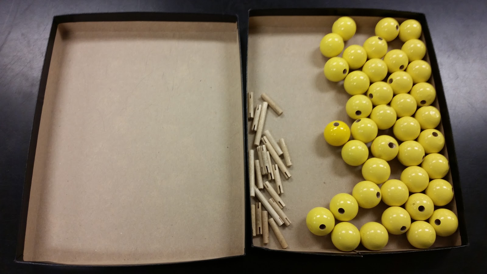
Figure 1: Initial set up for activity 1 experiment 1 2H ⇋ H2
When the timer begins, one student will be responsible for turning two model kit spheres into a single diatomic molecule. The other will be responsible for breaking apart any diatomic molecules into single atoms. One of the counters will count any formation of a molecule as a single event for the forward rate. The other counter will count any breaking apart of a molecule into two atoms as a single event for the reverse rate.
The teacher then sets a time for 5 or 6 minutes. An online timer displayed over a projector works great! Each minute the teacher calls out so that the counters start a new minute of data collection. At the end of the 5 or 6 minutes, everyone stops and the rates are totalled for each minute. Additionally, at the end, everyone must count how many H’s there are as well as how many H2 molecules are present. There can be 40 H’s, 20 H2 or any combination in between (IE 38 H atoms and 1 H2 molecule). These reflect the equilibrium concentrations.
At this point it is recommended to have the students make two whiteboards that show the rate vs. time for the forward and reverse reactions and the concentrations vs. time. For the first set of data collection there is often significant confusion with what to record and this will help address these issues before the bulk of data is collected. Common errors include counting the breaking apart of 1 molecule as 2 events, not recording equilibrium amounts and forgetting to start a new set of data at a minute interval.
Minutes
|
2H → H2
| |
Forward Rate
|
Reverse Rate
| |
1
|
13
|
13
|
2
|
12
|
12
|
3
|
14
|
13
|
4
|
14
|
15
|
5
|
15
|
15
|
Table 1: Sample data for Activity 1, experiment 1
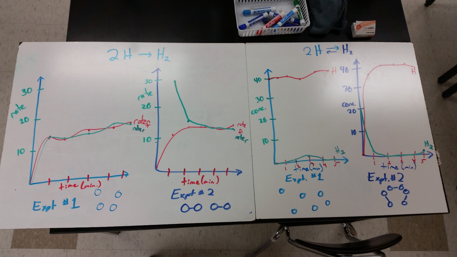
Figure 2: Sample whiteboards for activity 1 with model kits
Students should make a forward and reverse rate whiteboard that plots the rates at each minute interval. These plots should show that the forward and reverse rates are equal with some minor fluctuations throughout the experiment. The whiteboards give a good opportunity to define equilibrium via equal rates and to stress that the equal in equilibrium refers to the rates not the amounts. The students should verbalize via questioning that the reaction is still happening even though the amounts do not change because the rate that H2 is being formed is equal to the rate that H2 is being broken apart.
The concentration vs. time graph depends upon the level you seek to impart to your students. High-level students should be able to figure out how many H’s and H2 molecules there are after each minute has passed by comparing the rates of formation and destruction for each minute. If you are trying to reduce the time spent on this, this is a good chance to have students plot the initial and final equilibrium concentrations and have a simple curve to connect the two. If you spend more time on this part, emphasize that this is the graph that you can see and take data on in the lab, while the other graph is what we define equilibrium by but that rates are not visible to us except by the changes in concentrations.
After some good reflection and discussion from the first set of data the teacher should decide on how much time they wish to dedicate to the rest of this. If a lot of time is available the groups can all plot every graph. If less time is available the students can now collect the data for the remaining 5 trials and then whiteboarding can be split amongst the groups. For the next experiment, have all students set up 20 H2 molecules with the 40 model kit spheres and springs. The same experiment should be run, but the initial conditions have changed.
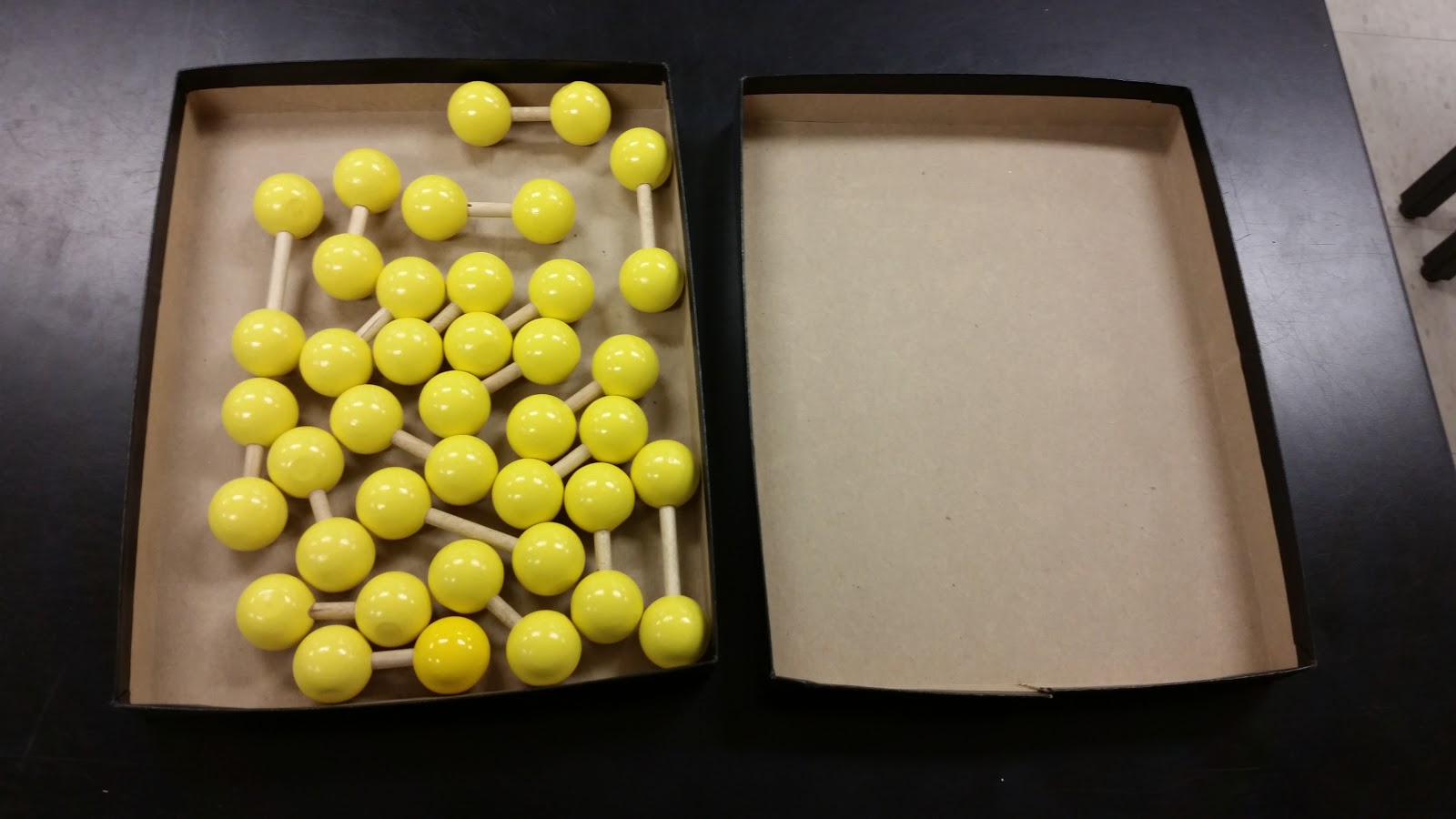
Figure 3: Initial setup for activity 1 experiment 2
Activity #2 - Rubber Bands (2R⇋ R2)

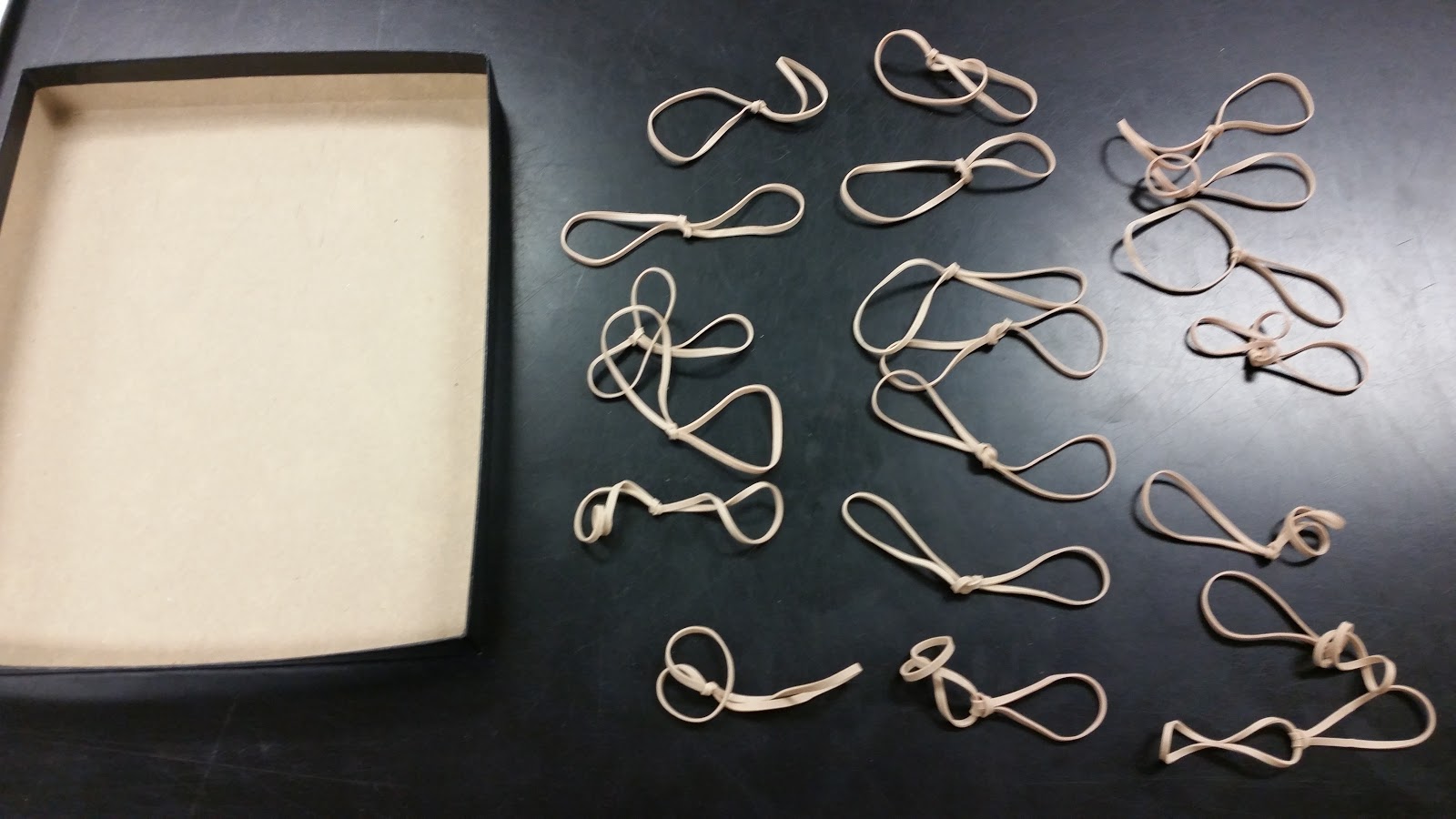
Figure 3: The initial setup for activity #2 Experiment 1 and Experiment 2
Students should count out 40 rubber bands. One student will tie them together, the other will take them back apart. This is a great example to follow up the model kits because the model kits are easy to take apart and really challenging to put together. Here the rubber bands are much easier to tie together than to take apart. When going through whiteboards this is a great time to have students verbalize that there is a relationship between the rates and the concentrations at equilibrium and connect back to kinetics. We are trying to emphasize that if a forward rate is much faster than the reverse, in order to achieve equilibrium you will need a lot of products and very little reactants. As you run out of reactants in the activity, that rate slows down because you there is nothing there to make products with. In the chemistry realm, as your reactants concentration decreases there are fewer collisions and this lowers the forward rate.
This is also a good opportunity to reflect on the fact that regardless of what you start with initially, at equilibrium you end up with similar distributions. For the model kits, you will achieve equilibrium with nearly all H’s and almost no H2 molecules because if you have a lot of H2 molecules the reverse rate will be too fast. For the rubber bands, you will achieve equilibrium with nearly all R2 molecules and almost no R atoms because if you have a lot of R atoms the forward rate will be too fast. This can be summarized using rate laws quite nicely. Let’s start with the model kits.
Ratef = kf [H]2
We know that the forward rate is very slow regardless of [H]. This means that kf is small. The reverse rate can be represented by:
Rater = kr[H2]
We know the reverse rate is very fast unless we severely limit the [H2]. If students question the exponents used, we can justify by mechanisms since each reaction is a single elementary step and thus is the rate-determining step.
Because kf is very small and kr is very big and at equilibrium the opposing rates are equal by definition, we can put this into very simple terms for students.
Ratef =Rater
kf [H]2 = kr[H2]
kf / kr = [H2]/[H]2
kf / kr = [H2]/[H]2
Because the reverse rate is faster than the forward, there must be significantly more [H] than [H2] to achieve equilibrium. For rubber bands we see the opposite:
kf / kr = [R2]/[R]2
Because the forward reaction is so much faster, there must be significantly larger amounts of product to achieve equal opposing rates and equilibrium. This would be an appropriate time to define the equilibrium constant to simplify these discussions. It can be defined by the rate constants, the concentrations of products over reactants, or both.
Activity #3 - Paper Clips (2P ⇋ P2)
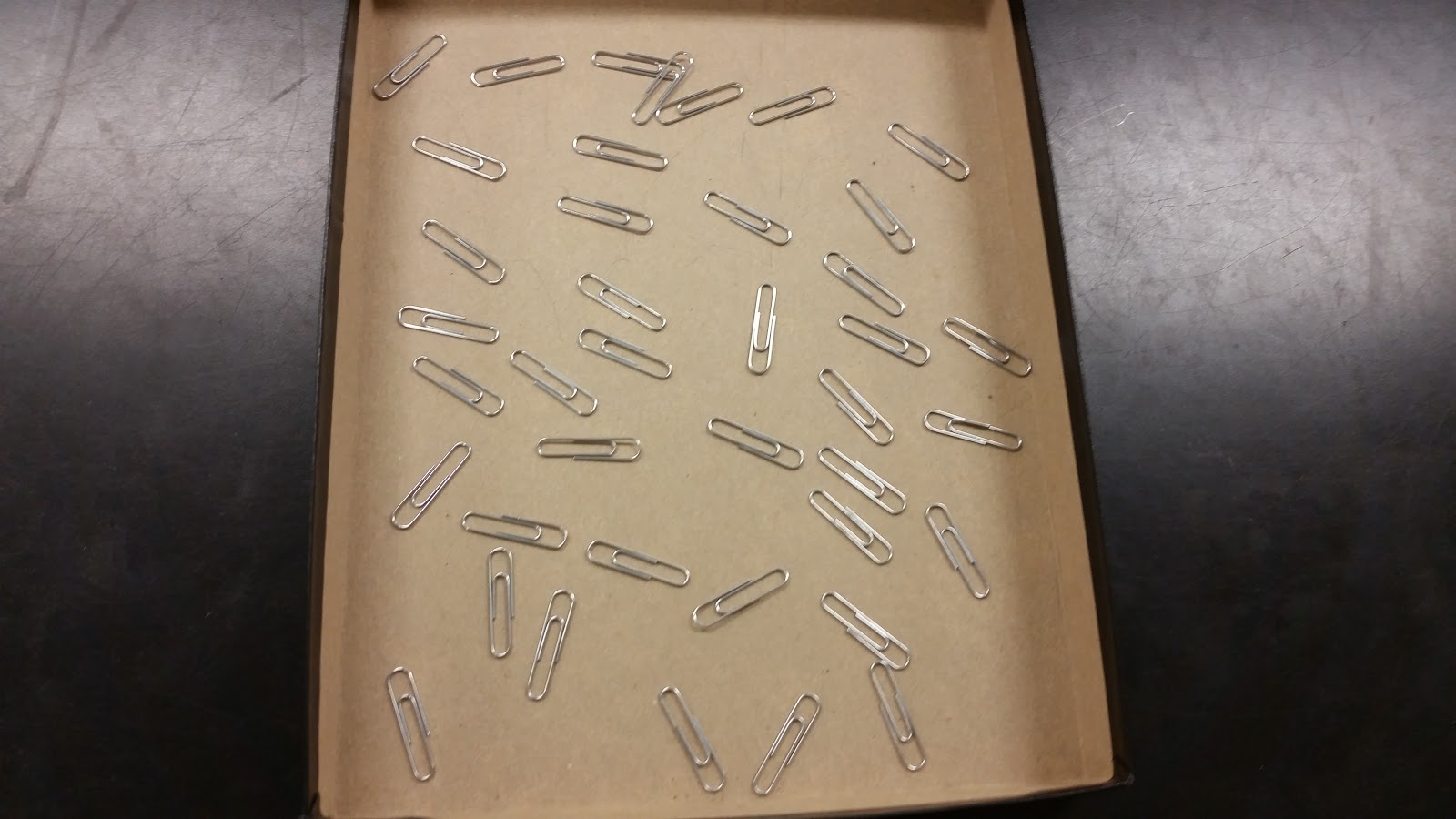
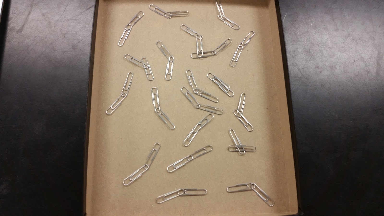
Figure 4: Inital setup for activity #3 experiment 1 and experiment 2
The final activity has students get 40 paper clips in trial 1. In trial 2 the students should start with 20 P2 molecules and no unlinked paper clips. One student links two paper clips to form a diatomic P2 molecule. The other unlinks the two. This activity is meant to be opposing rates that are not significantly biased one way or another. The model kits always favor the reactants, the rubber bands almost always favor the products. This depends on the students and style and can favor either. Ideally there is balance at equilibrium, but often equilibrium will not be achieved in this final activity.
Whiteboarding, Data Analysis and Discussion
After all six trials are completed, students should have rate data and equilibrium data for all three activities starting with all reactants and all products. The discussion should have targets, but also should allow students to really explore the connections between rates and concentrations before equilibrium is achieved and after equilibrium is achieved. Here are some potential targets for the conversation that ensues.
Target #1 - At equilibrium, the reaction is still occurring, but the opposing rates are equal and so the concentrations are constant.
Target #2 - If the forward or reverse rate is significantly slower or faster than the opposing rate, a large concentration difference is needed to achieve equilibrium. (A great question to ask is if there are way more products at equilibrium, which rate is faster with equal concentrations, have students justify using one of the activities as an example)
Target #3 - Concentrations are easily measured in labs, rates derive from the changes in concentration and are not “visible” in the same manner. These activities allow us to “see” rates that we cannot do with chemical processes in the same direct manner.
Target #4 - The equilibrium constant, K, can be used to describe the concentrations at equilibrium. If K is large, mostly products are present at equilibrium. If K is small, mostly reactants are present at equilibrium.
Target #5 - Graphs of rate vs. time will show when equilibrium is achieved when the rates are equal to each other. At the high end level, stoichiometric ratios of rates can also be developed here (IE, if we track the rate of formation of H or H2, the rate will differ by a factor of 2). The graphs are often broken up into an equilibrium region and a kinetic region.
Target #6 - Graphs of concentration vs. time will show when equilibrium is achieved when the concentrations become constant.
Target #7 - The initial amounts have no limits, the equilibrium amounts are limited by K and the changes in amounts are restricted by stoichiometry.
Target #8 - Now would be an appropriate time to introduce the reaction quotient Q. If we plug in concentrations and determine we have too much product or reactants, we can determine how the rates will cause the reaction mixture to change to achieve equilibrium. This is a great way to start Le Chatelier’s Principle without having to just hand wave about stresses.
Tips for success
- It is easier and more effective to have the teacher set a timer and call time off. Otherwise you will have many mistakes in many groups where students forget to reset the rates each minute.
- It is better to do 1 set of data collections as a group and analysis so students understand the end goal and mistakes are limited to a single trial. If you have students collect all of the data before doing any analysis, at least one group will have done something incorrectly and will not have useful data.
- Distribute rubber bands and collect immediately after use.
- Take pictures of the whiteboards and use them in later topics such as Le Chatelier’s Principle, thermodynamics, acid-base, vapor pressure and reaction energy diagrams.
- Have students use the top cover so they have two containers for model kits to be in and this will help limit spills onto the floor.
- Doing calculations such as K, Q for the activities can be great for connecting the concepts into how we will do chemical analysis of equilibrium, but do not do this at the expense of connecting rates and concentrations.
Follow up assessment questions:
Two sealed containers of different volumes are shown below.
A B
Container A and B both have liquid water present at the same temperature. Some of the liquid water has evaporated and formed steam according to the following equation:
H2O (l) ⇋ H2O (g)
The vapor pressure in both containers is the same and constant.
- Even though the vapor pressure is constant in container A, the forward and reverse processes are still occurring, just at equal rates.
- Draw in particles in container A that are undergoing both processes.
b. The forward rate represents evaporation of the liquid particles, what does the reverse rate represent?
c. In container B, there is a smaller surface area of the water and therefore a slower rate of evaporation. How does the reverse rate in container B compare to the reverse rate in container A?
d. Assume the liquid in container B is heated, what will happen to the forward rate?
e. What will happen as container B is heated in order to achieve equilibrium again at the new higher temperature?
Additional Equilibrium Questions:
FRQ #13 + solution