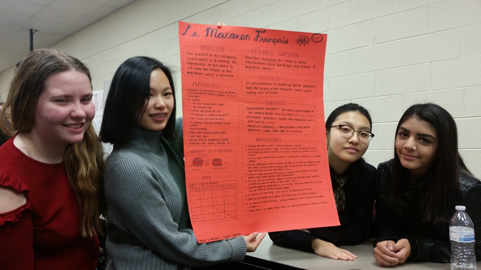
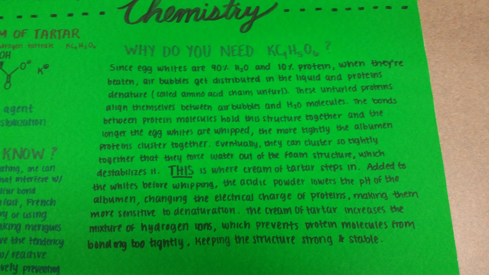
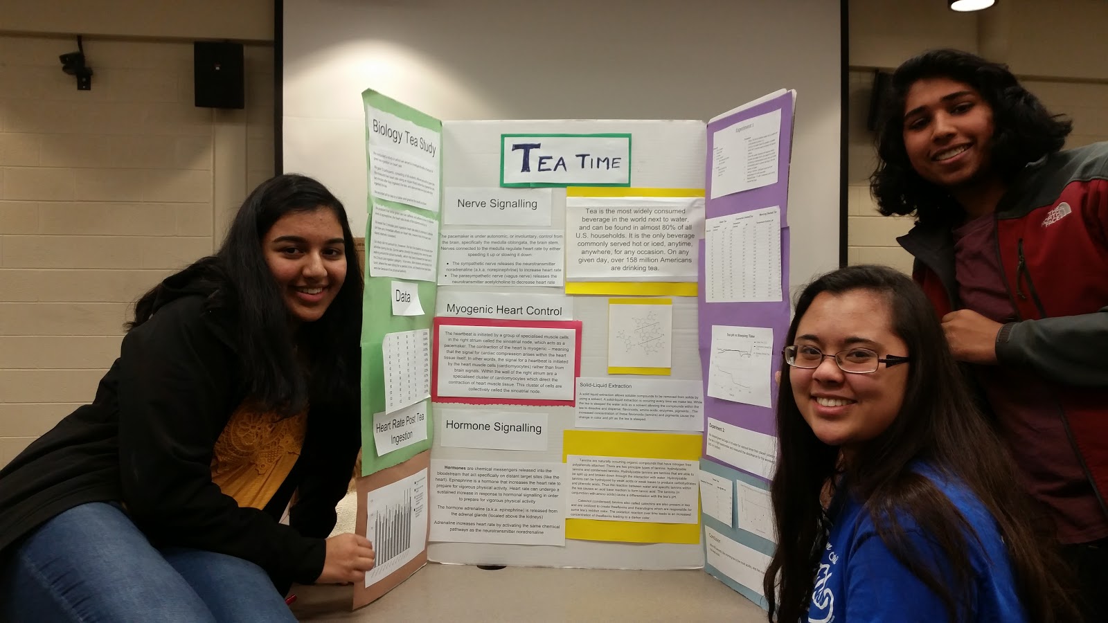
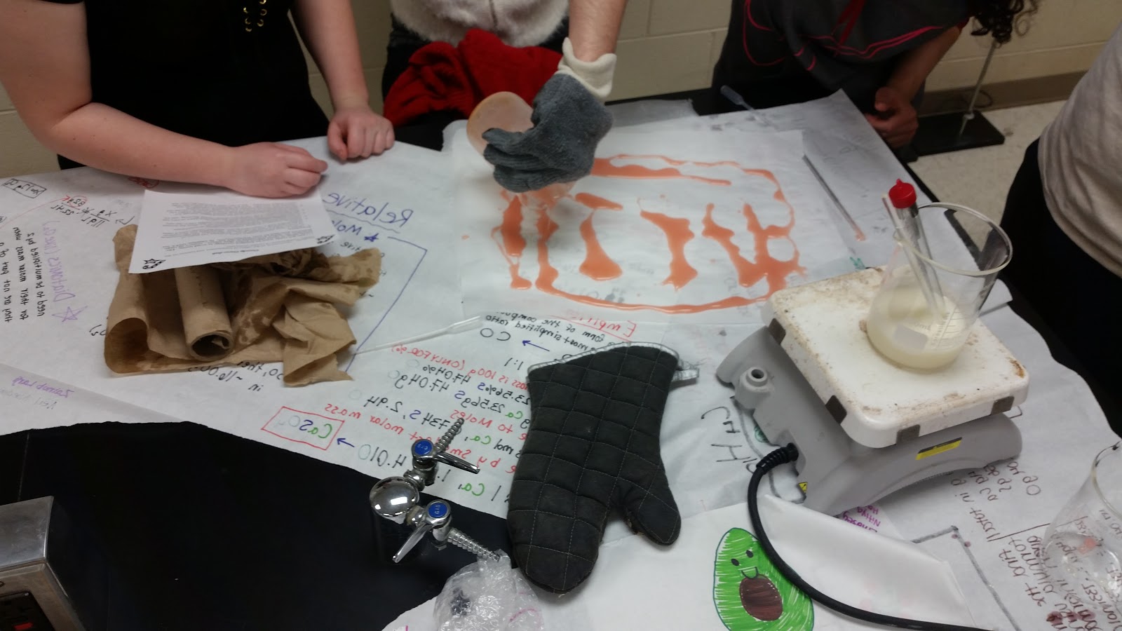
IB students were tasked with creating an experiment or set of experiments that analyzed international foods from different scientific perspectives (usually biology and chemistry). Students used a variety of experimental methods utilizing creativity in their methods. Pop Rocks (Spain) were dissolved in a hydroxide solution and then titrated to measure the amount of carbon dioxide present (Figure 14). Another group tested the various components of Bakkalava to determine which had the biggest impact on the boiling point of the mixture (Figure 1). One group tested how to make the perfect macaron (Figure 4, Figure 5). They detailed the mechanism by which potassium bitartrate influences the protein structures and how this affects the texture and height. Students used tea to investigate caffeine and tannin amounts, then connected these experiments with biology by examining heart rate after consumption (Figure 6).
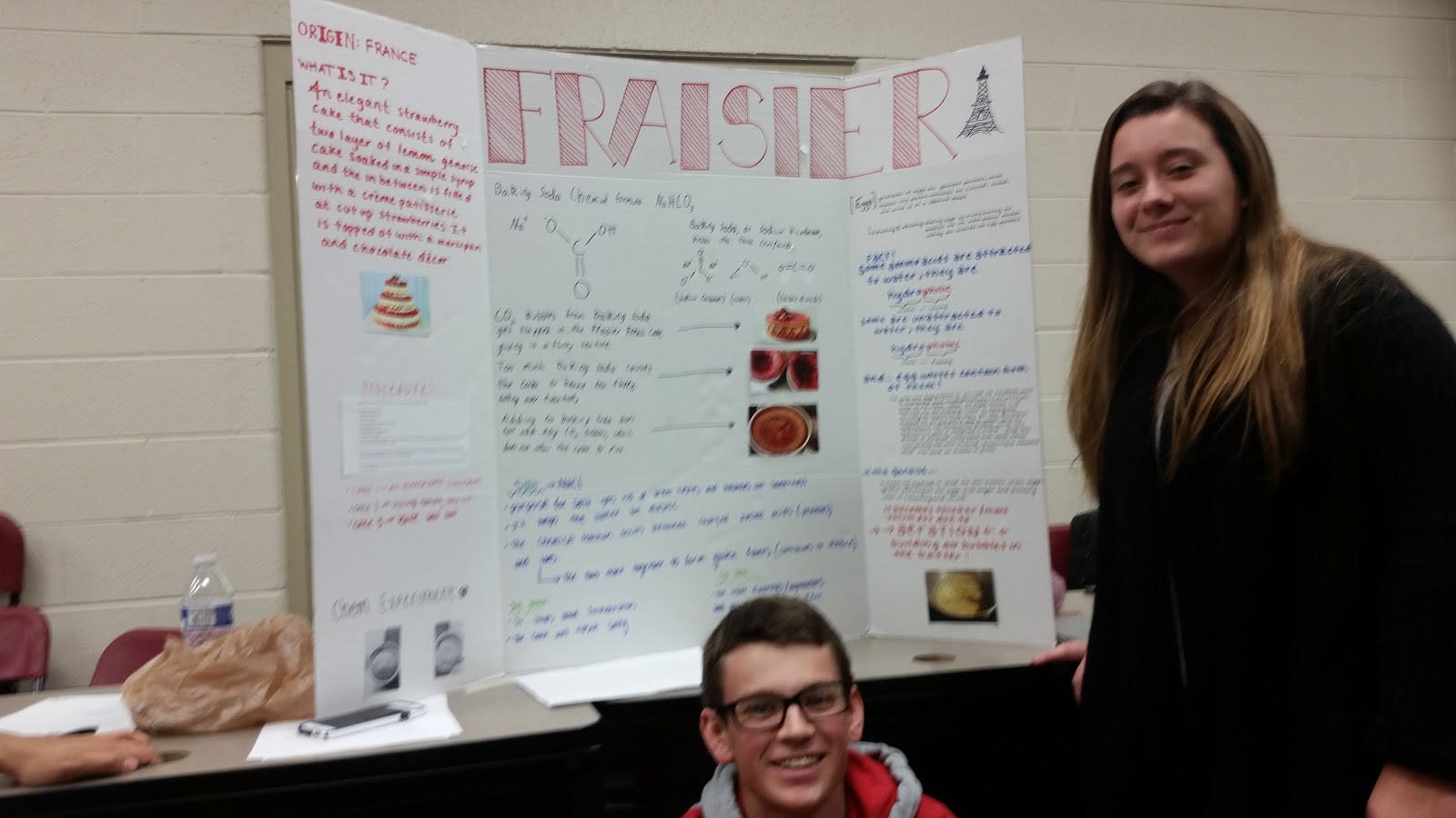
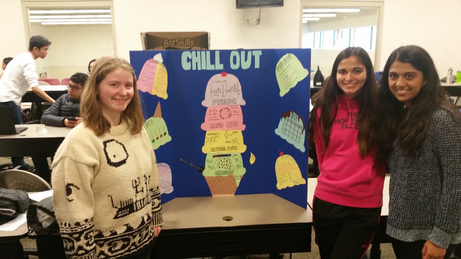
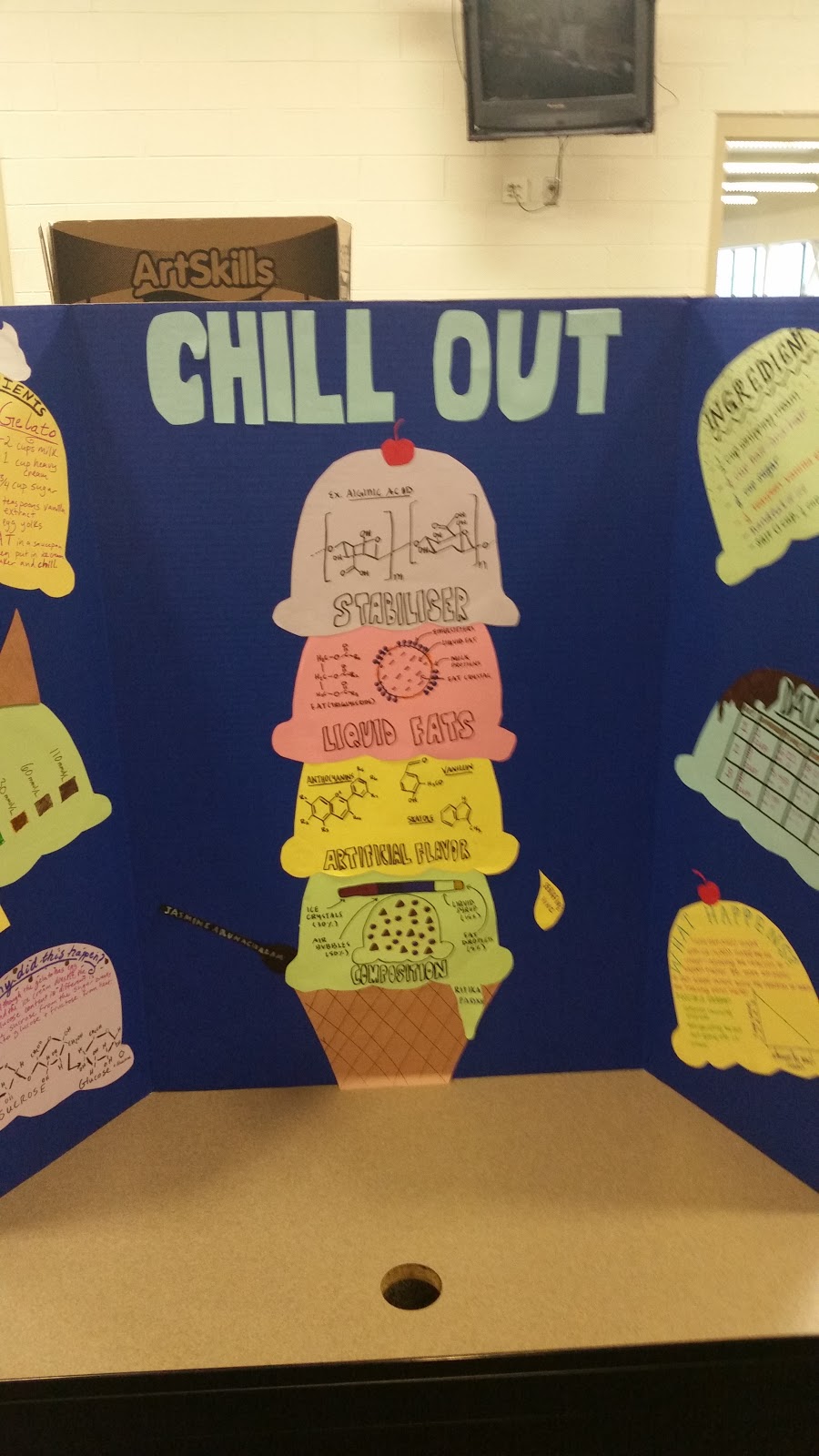
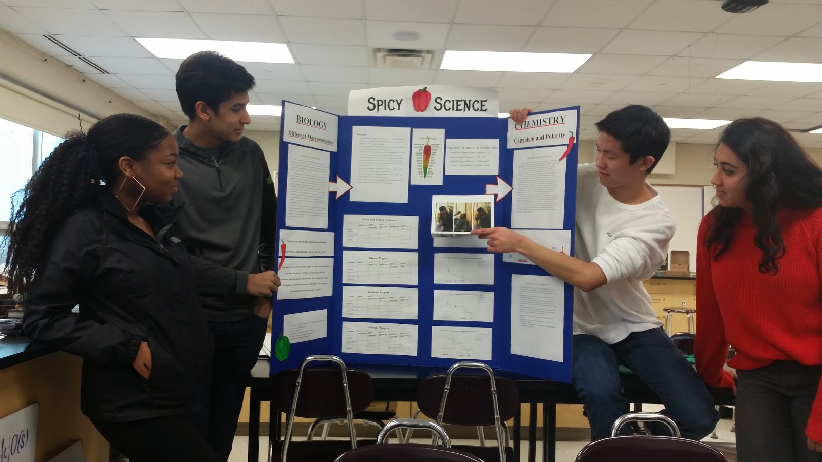
Students testing dough and yeast (Figure 7) found great data showing how yeast affected the rise of the dough (Figure 8). Students gathered some brave volunteers to test which foods (Figure 13) reduced the affects of capsacain in spicy foods (peanut butter was typically the best). Students made Fraisier (French strawberry cake) with varying amounts of baking soda (Figure 9). Students tested textures of various foods after a variety of experiments to simulate cooking (Figure 2, Figure 3, Figure 10). And even though students researched ice cream and gelato (Figure 11, Figure 12) we still spent the next day making candy canes (Figures 15-17). During our candy making one group even added in citric acid and ended up with sour gummy candy that was delicious.
Figure 1: Chemistry and Biology of Bakkalava
Figure 2: Chemistry and Biology of kibbeh
Figure 3: Chemistry and Biology of noodles
Figure 4: Chemistry and Biology of macarons
Figure 5: Protein denaturing, air bubbles and cream of tartar for the perfect macaron
Figure 6: Chemistry and Biology of Tea
Figure 7: Chemistry and Biology of yeast and dough
Figure 8: Great correlation between dough rising and increasing quantities of yeast
Figure 9: Chemistry and Biology of Fraisier
Figure 10: Chemistry and Biology of seviche
Figure 11: Chemistry and Biology of Ice Cream
Figure 12: Anthocyanins, skatole, alginate stabilizers and other relevants structures for ice cream
Figure 13: Chemistry and Biology of spicy
Figure 14: Chemistry and Biology of Pop Rocks
Figure 15: A batch of candy cane mix now ready to shape and color
This experiment uses inquiry and modeling techniques to develop an understanding of why transition metal aqueous solutions are colorful using d-orbital splitting when ligands and transition metal ions form complex ions. Students must have learned basic quantum theory especially understanding that absorbing light corresponds to a change in motion of the electron where the electron moves to an excited state of higher energy and when light is emitted the electron changes to a lower energy state. It may be helpful, but not necessary for them to have done calculations of light energy, frequency and wavelength as well as be familiar with the electromagnetic spectrum.
Day 1
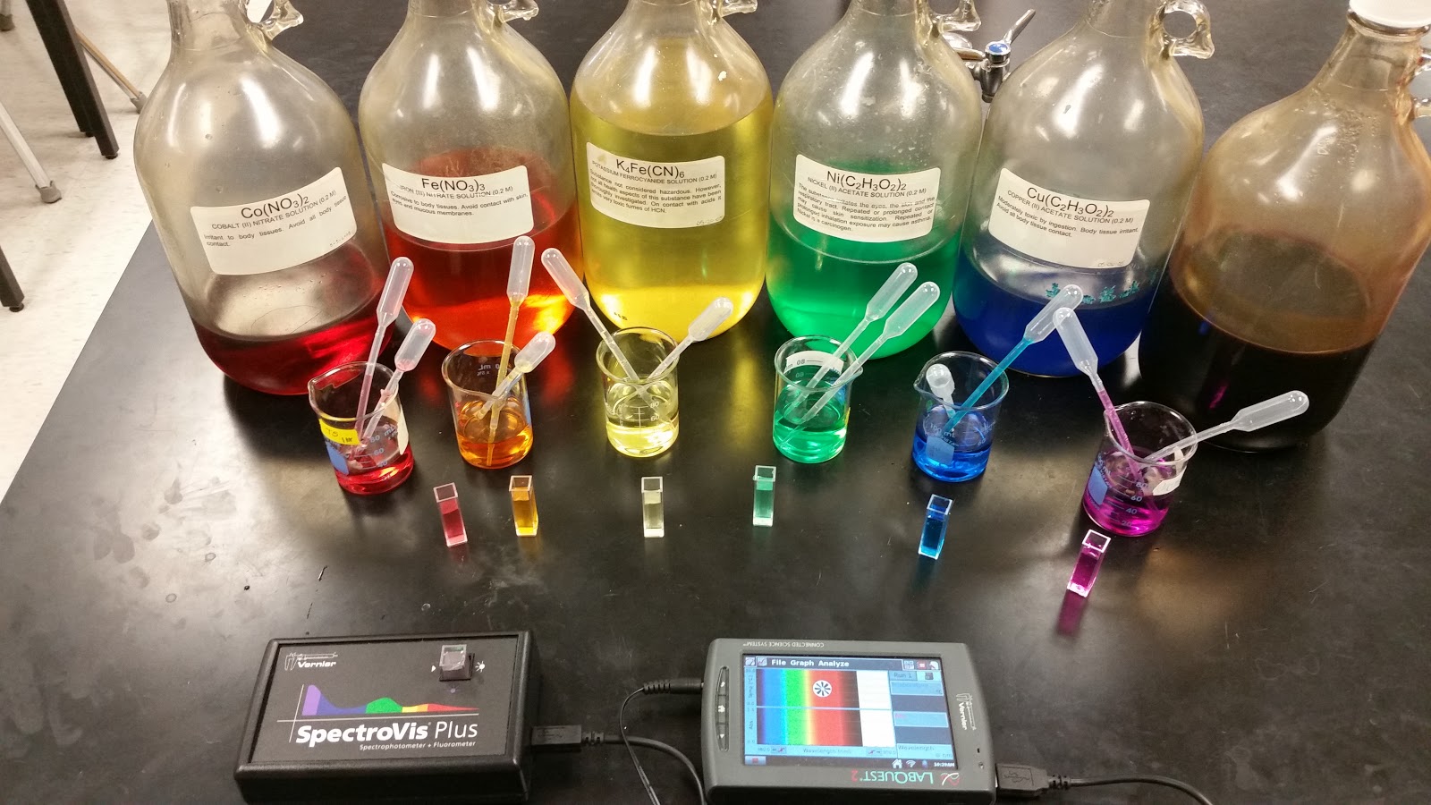
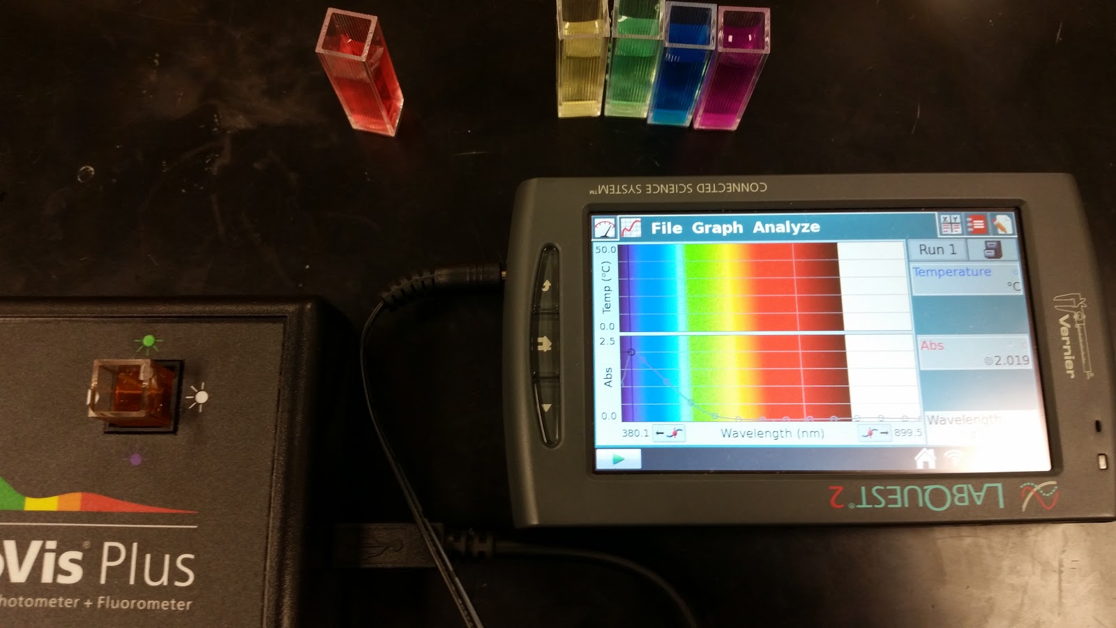
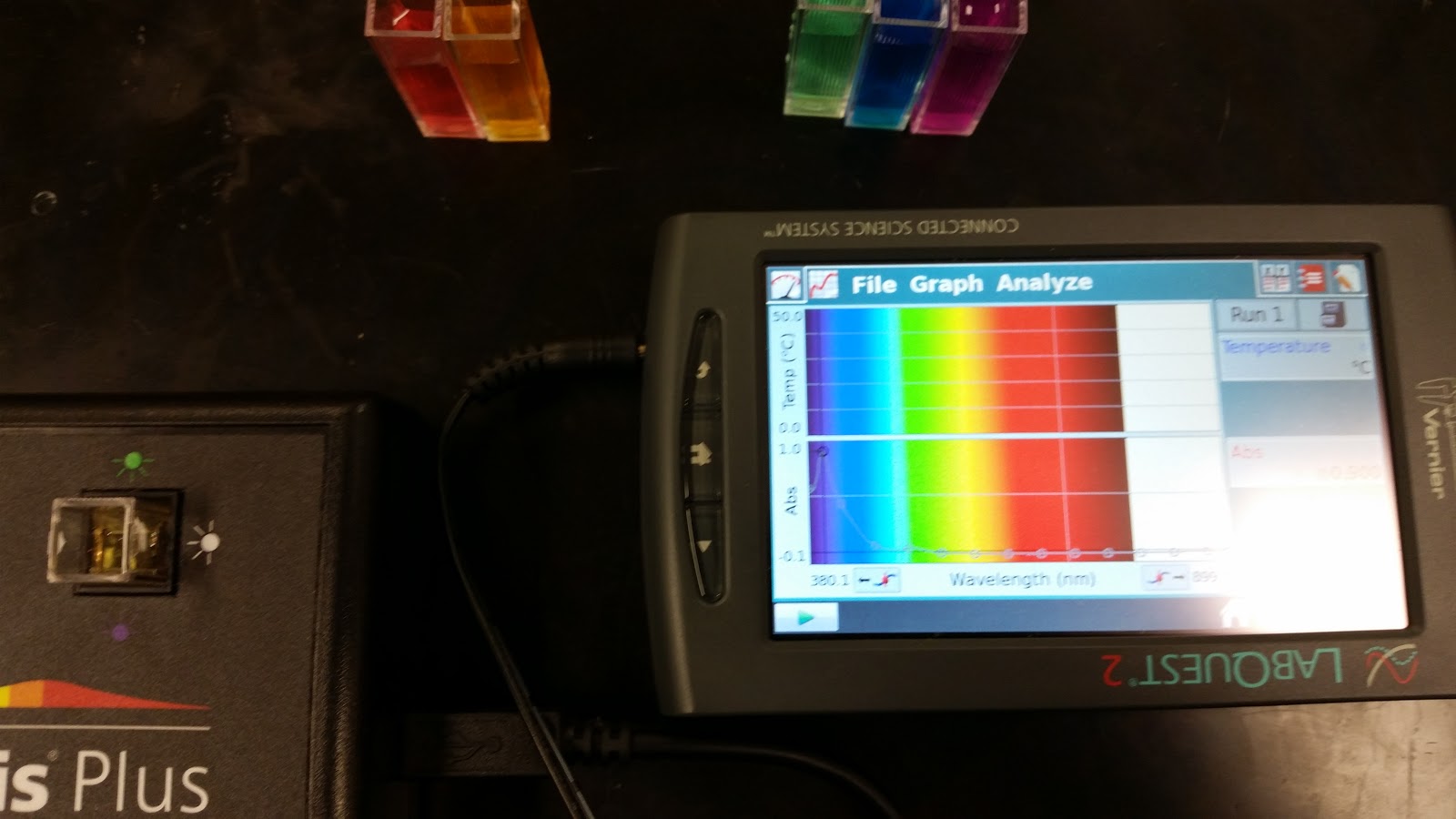
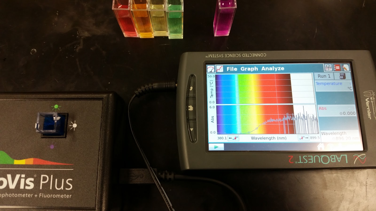
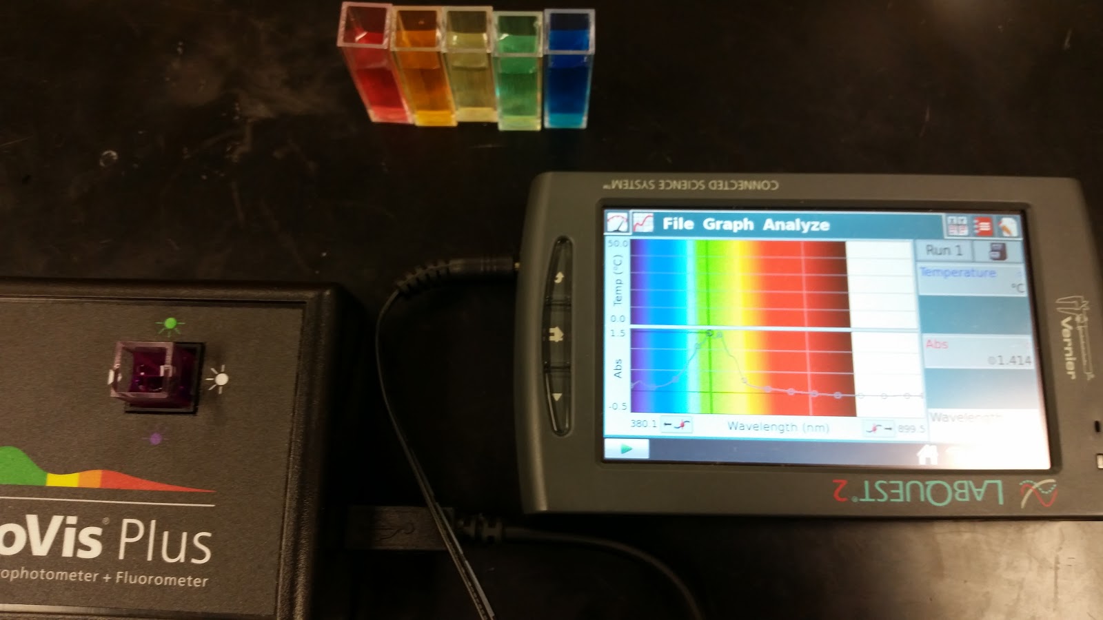
The students are instructed on how to utilize the Vernier Spectrovis Plus equipment. They are briefed on how to fill cuvettes to about ¾ full, to hold the cuvettes on the ridged side so as not to leave smudges, how to calibrate the spectrophotometer and the correct settings. The data they are instructed to collect is the principal color or colors that are absorbed and which colors are transmitted. The chemicals used were Co(NO3)2, FeCl3, K4Fe(CN)6, Ni(C2H3O2)2, Cu(C2H3O2)2 and KMnO4. The anions used are not important, but it is helpful to have at least two with the same anion to eliminate the possibility of the color being dictated by the anion. A small amount of chemical is needed for the entire class and can easily be reused from year to year if put into containers that can be sealed. The solutions used were 0.2 M because that is what we had already made for previous labs. The KMnO4 solution was diluted to an unknown concentration so the absorbance was more reasonable. The concentration should not be too high or the absorbance will be beyond the measuring apparatus.
Figure 1: The experimental setup used for colorful salts
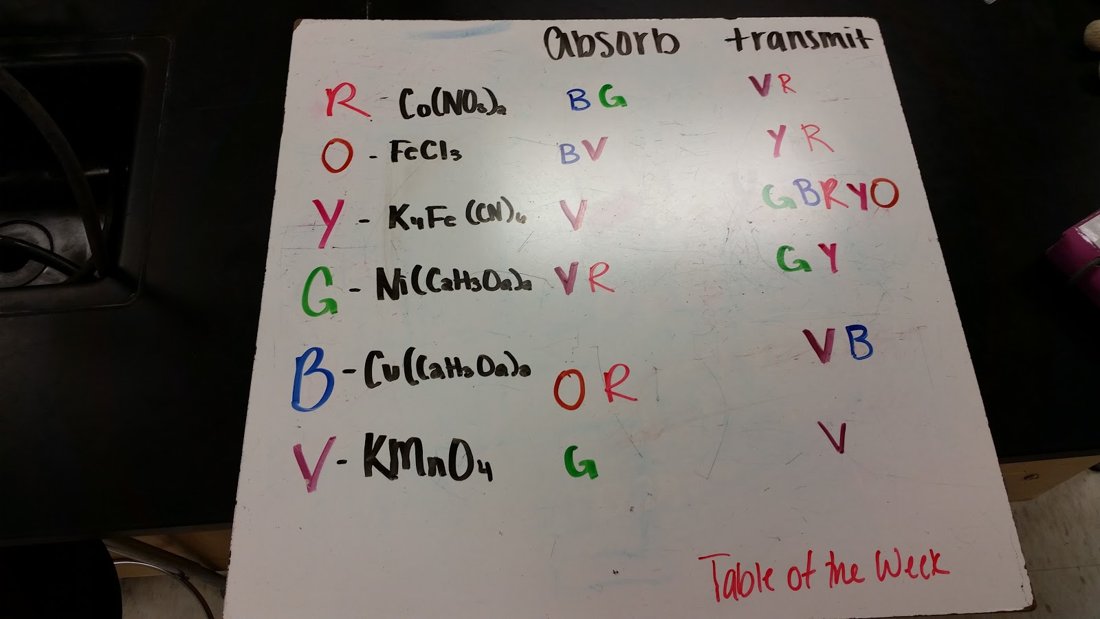
Students then ran all of the solutions and compiled their data into whiteboards.
Figure 2: Student data from the colorful salts experiment
Discussion
At this point the discussion began analyzing the data collected. There was not sufficient time for the entire discussion in the first period, but that worked out very well. There were two keys that I wanted to establish from the experiment and a cliffhanger for the following lesson. The first discussion point was that when a solution is (any color) it will transmit _____ and absorb ______. We first try and build an understanding of what we are seeing. If a solution is red, that means that the solution transmits red light and absorbs complementary colors such as green or blue. The second key for day 1 is to begin analyzing what each solution has in common so that we can develop a model to explain what is happening. In our first class of this we came up with the fact that the six solutions have the following in common (ionic, transition metal, metals and nonmetals are present in all six solutions, all metals are from period 4). This is a good time to briefly mention that the color must be from the cations since some anions are the same and the colors differ. The final component of day 1 is to preview that the next lesson will involve constructing a model to explain what is happening that makes these solutions colorful in the way that they are. We would like to use their commonalities to provide an explanation of the observed phenomena.
Day 2
Discussion
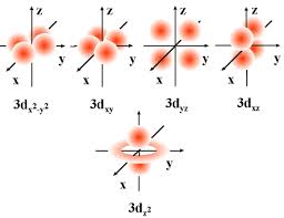
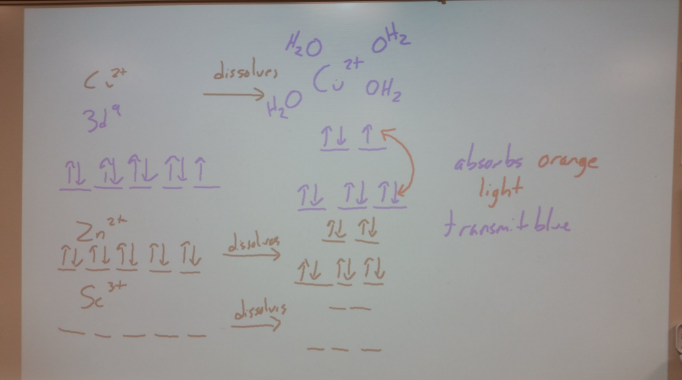
Day 2 began with our list of commonalities of our six solutions. I started class by saying that our list was insufficient and we must add to it. We then added that each solution was aqueous and that they were all colorful. At this juncture it was now time to begin developing a model. I brought out a solution of zinc nitrate to show that it was colorless and I also informed students that Sc(NO3)3 is also colorless. This is a good time for students to discuss in their lab groups what is needed for the solutions to be colorless. Someone should conclude that a partially filled set of d-orbitals is required. This is a key point and should be written down. It should also start the next question. The students are aware that in order to absorb light, an electron must move from one state (orbital) to another. Where are the 3d electrons moving to? And why can’t the 3d shell be full or empty? Now draw a set of 5 orbitals on the board to highlight this. At this point I reminded students that there are shapes of the d-orbitals and showed an image of them.
Figure 3: 3d orbitals from wikipedia
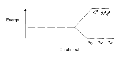
The images are best if they show axes and you can point out that some are along the axes (2) and some are between them (3). These orbitals all have the same energy, but will be influenced differently by the negative charge of ligands when forming a complex ion. Since all 6 solutions are aqueous, the water molecules have the oxygen end surrounding the transition metal ions. These water molecules are going to cause the d-orbitals to go from being 5 degenerate states to splitting into two groups. This splitting is what is key for the colorful transition metal cations.
Figure 4: d-orbital splitting from wikipedia
Now is a good time in the discussion to revisit Zn2+ being colorless and Sc3+ being colorless. The zinc ions have the electron configuration of 3d10. This will fill all 5 orbitals even when split and thus no transitions can occur from the bottom 3 to the top 2. For Sc3+ the electron configuration has no electrons in the d-shell and thus there are no electrons to shift from the bottom to the top. It is only when the d-shell is partially filled that the splitting causes colors of light to be absorbed.
Figure 5: Summary board at the end of our discussion
Figure 6: Whiteboard after going through zinc ions and scandium (III) ions being colorless
At this point we organize our model. When transition metal ions with partially filled d-orbitals are surrounded by a ligand (with negative charge)
The d-orbitals split into different energies based on the proximity of the ligands
The electrons can move between these new split levels absorbing visible light
The color of the resulting solution is the light being transmitted
The color is the complement of the light being absorbed
This does not happen for Sc3+ or Zn2+ since the d-orbitals are either empty or completely full
To test our new model, we can then substitute other ligands in place of water to show that ligands with different amounts of negative charge and different proximity will cause a variety in the splitting of energy. Thus color will change when copper (II) ions have excess ammonia or chloride added.
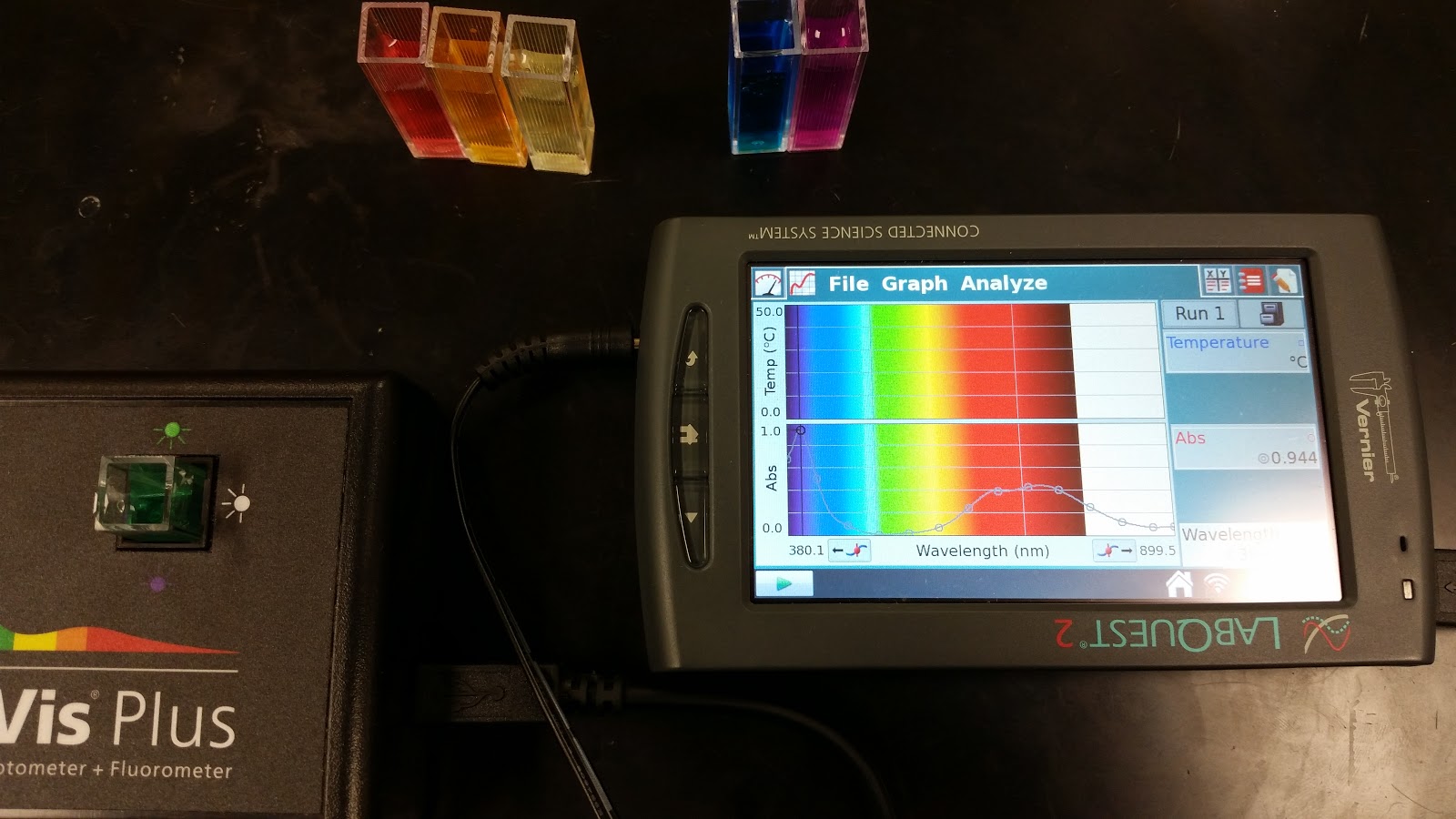
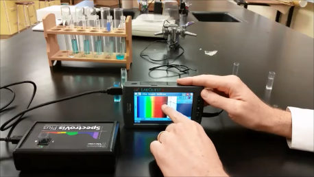
If you would like to do this activity but do not have the Vernier equipment, you are welcome to utilize the video of the experiment and I also am placing photos of the absorbance curves below.
Figure 7: Red solution Co(NO3)2 absorbs blue and green light
Figure 8: Orange solution (FeCl3) ab
Figure 9: Yellow solution (K4Fe(CN)6) absorbs violet and blue light
Figure 10: Green solution (Ni(C2H3O2)2) absorbs red and violet light
Figure 11: Blue solution (Cu(C2H3O2)2) absorbs red and orange light
Figure 12: Violet solution (KMnO4) absorbs green and yellow light
Additional explanation for students can be found here:
A copper (II) sulfate of unknown concentration is prepared for each lab group. The solutions are then distributed where each group gets slightly more than 50 mL of solution to analyze and determine the concentration of in two manners.
Figure 1: 0.50 M solution of CuSO4 (middle) with two solutions with unknown concentration
Day 1:
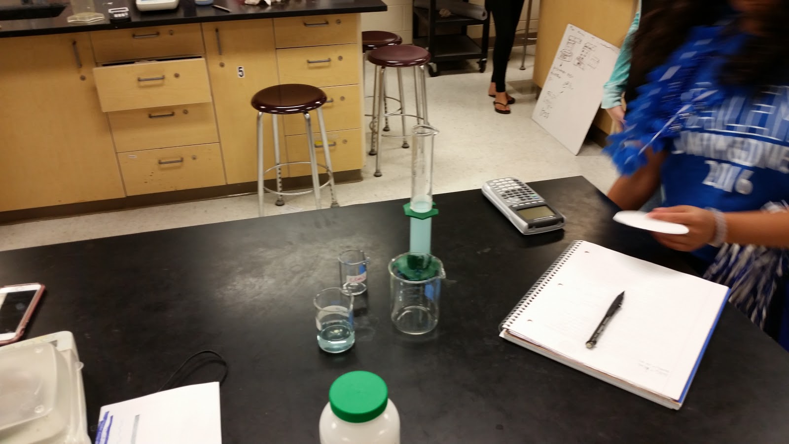
After students receive their samples they should separate a large portion of their solution to mix with 0.2 M barium nitrate solution. This forms the barium sulfate precipitate that can be separated via filtration as shown below.
Figure 2: The graduated cylinder contains the unknown solution after mixing with barium nitrate
Figure 3: The mixture is now ready to filter, wash and dry
Day 2:
Today the students prepare a set of solutions with varying concentration to construct a calibration curve. The students have 0.50 M CuSO4 solution and distilled water. It is up to them to determine what an acceptable range of concentration is given the parameters that the highest and lowest possible concentrations are 0.08 M to 0.001 M for the unknown solutions. Today the students are also instructed on how to use the Vernier spectrophotometers to produce a line of best fit from their calibration curve. They are taught how to calibrate the spectrophotometer with distilled water, how to handle the cuvettes, how to select the appropriate wavelength of light for analysis, how to construct the calibration curve and finally how to produce a line of best fit for their data. Students may obtain the mass of their precipitate from day 1 at this point. Any errors in washing should be fixed today.
Figure 4: The spectrophotometer can be used to determine the appropriate wavelength for analysis, in this experiment red light near 700 nm is a good choice
Day 3
Students continue making solutions, testing the solutions with the spectrophotometers and begin calculations for their experiments. Students may re-mass their precipitates from day 1 again to confirm no water was present on day 2. Calculations should show how the concentration in molarity was determined in both experiments and should comment on the answers produced by both methods and what errors occur in each that make one method superior to the other. Video of the experiment